任务优化的循环神经网络建模 引言 这里,我们基于人工神经网络的方法构建循环神经网络。学习人工神经网络或深度学习,不仅是当今机器学习的主导框架,对计算神经科学而言也是一个有用的工具。
深度学习本身可能并不符合生物现实。然而,深度学习最终的结果可能是有用的大脑模型(不保证,但是可能)。由于人工神经网络的复杂性,它们可以模拟复杂的行为和神经活动。
从优化的角度来说,人工神经网络建模可以提供规范性解释,即为什么一个网络可以以某种方式完成某个任务,因为我们可以设计目标函数,类似于生物进化的视角。
任务介绍
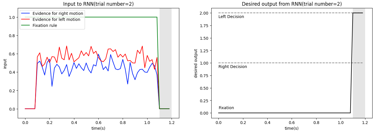
双向强迫选择任务PerceptualDecisionMaking ,被试需要整合两个刺激来决定哪一个刺激的平均水平更高。参数介绍: dt:Timestep duration. (def: 100 (ms) int)rewards:
R_ABORTED: given when breaking fixation. (def: -0.1 float) R_CORRECT:given when correct. (def: +1. float) R_FAIL:given when incorrect. (def: 0. float)
timing:Description and duration of periods forming a trial.stim_scale:Controls the difficulty of the experiment. (def: 1., float)cohs:list of float, coherence levels controlling the difficulty of the tasksigma:float, input noise leveldim_ring:int, dimension of ring input and output
环境配置
NeuroGym 是一个精选的神经科学任务集合,具有统一的接口。其目标是促进关于神经科学任务的神经网络模型的训练。Google Colab 是一个基于云端的免费Jupyter笔记本环境,为用户提供了方便、免费的编码环境,并具备强大的计算资源和协作功能,适用于数据科学家、研究人员和机器学习工程师等进行代码开发、实验和协作。1 2 3 4 5 6 7 8 9 10 11 12 13 14 15 16 17 18 19 20 21 22 23 ! git clone https://github.com/gyyang/neurogym.git %cd neurogym ! pip install -e . import time import numpy as np from matplotlib import cm import matplotlib as mplimport matplotlib.pyplot as pltfrom matplotlib.colors import ListedColormap, LinearSegmentedColormapfrom matplotlib.lines import Line2Dfrom IPython import display import gym import neurogym as ngym import torch import torch.nn.functional as Ffrom sklearn.decomposition import PCA from scipy.special import softmaxmpl.rcParams.update(mpl.rcParamsDefault)
模型概览
$x(t)$:输入变量
$r(t)$:循环变量
$o(t)$:输出
$W_x$:输入权重【可训练】
$W_r, b_r$:循环权重 & 偏置
$W_o, b_o$:输出权重 & 偏置
$\alpha=\frac{\bigtriangleup t}{\tau }$
此外,在人工神经网络建模中,我们可以使用各种各样的激活函数,比如ReLU、sigmoid和softplus函数。
1 2 3 4 5 6 7 8 9 10 11 12 13 14 15 16 17 18 19 20 hpar = dict ( dt = 20 , stim_len = 1000 , stim_noise = 0.3 , seq_len = 60 , n_neurons = 64 , network_noise = 0.1 , tau = 100 , activation_fun = 'relu' , batch_size = 16 , n_iteration = 1000 , learning_rate = 0.01 , optimizer = 'Adam' , loss = 'CrossEntropy' )
batch:指每次迭代中用于训练模型的样本数量。批大小的选择会影响训练的效果和速度。较大的批大小可以提高训练的效率,因为可以同时处理更多的样本,但会消耗更多的内存。较小的批大小可以提供更多的随机性和模型收敛的稳定性,但可能会导致训练时间增加。iteration:指完成整个训练数据集的一次遍历。迭代的数量取决于训练数据集的大小和训练过程的要求。通常,较大的数据集需要更多的迭代来使模型收敛,而较小的数据集可能需要较少的迭代。
训练 RNN 执行任务 1 2 3 4 5 6 7 8 9 10 11 12 13 14 15 16 17 task_name = 'PerceptualDecisionMaking-v0' kwargs = {'dt' : hpar['dt' ], 'timing' : {'stimulus' : hpar['stim_len' ]}, 'sigma' : hpar['stim_noise' ]} env = gym.make(task_name, **kwargs) dataset = ngym.Dataset(env, batch_size=hpar['batch_size' ], seq_len=hpar['seq_len' ]) inputs, target = dataset() print ('Input to network has shape(SeqLen,Batch,Dim)=' , inputs.shape)print ('Target to network has shape(SeqLen,Batch)=' , target.shape)
gym.make(task_name, **kwargs):是OpenAI Gym库中用于创建一个与特定任务相关的环境对象。task_name表示要创建的任务的名称,例如CartPole-v1,每个名称对应一个特定的任务环境。**kwargs是一个可选的关键字参数,用于传递额外的配置选项给环境。**用于将一个字典(dictionary)解包为关键字参数传递给函数。字典的关键字需与函数的参数名称匹配,参数顺序可以改变。
1 2 3 4 5 6 7 8 9 10 11 12 13 14 15 16 17 18 19 20 21 22 23 24 25 26 27 28 29 i_trial = np.random.choice(hpar['batch_size' ]) end = sum ([v for _,v in env.timing.items()])/1000 times = np.arange(end, step=env.dt/1000 ) rules = end - env.timing['decision' ]/1000 , end f, ax = plt.subplots(1 , 2 , figsize=(16 ,5 )) ax[0 ].axvspan(rules[0 ], rules[1 ], facecolor='grey' , alpha=0.2 ) ax[0 ].plot(times, inputs[:,i_trial,1 ], 'blue' , label='Evidence for right motion' ) ax[0 ].plot(times, inputs[:,i_trial,2 ], 'red' , label='Evidence for left motion' ) ax[0 ].plot(times, inputs[:,i_trial,0 ], 'green' , label='Fixation rule' ) ax[0 ].set_ylabel('input' ) ax[0 ].set_ylim([-0.1 ,1.1 ]) ax[0 ].legend(loc='upper left' ) ax[0 ].set_xlabel('time(s)' ) ax[0 ].set_title(f'Input to RNN(trial number={i_trial} )' ) ax[1 ].axvspan(rules[0 ], rules[1 ], facecolor='grey' , alpha=0.2 ) ax[1 ].hlines(y=1 , xmin=times[0 ], xmax=times[-1 ], color='gray' , linestyle="dashed" ) ax[1 ].hlines(y=2 , xmin=times[0 ], xmax=times[-1 ], color='gray' , linestyle="dashed" ) ax[1 ].text(0 , 0.08 , 'Fixation' ) ax[1 ].text(0 , 0.9 , 'Right Decision' ) ax[1 ].text(0 , 1.9 , 'Left Decision' ) ax[1 ].plot(times, target[:,i_trial], 'k' ) ax[1 ].set_ylabel('desired output' ) ax[1 ].set_ylim([-0.1 ,2.1 ]) ax[1 ].set_xlabel('time(s)' ) ax[1 ].set_title(f'Desired output from RNN(trial number={i_trial} )' ) plt.show()
1 2 3 4 5 6 7 8 9 10 11 12 13 14 15 16 17 18 19 20 21 22 23 24 25 26 27 28 29 30 31 32 33 34 35 36 37 38 39 40 41 42 43 44 45 46 47 48 49 50 51 52 53 54 55 56 57 58 59 60 61 62 63 64 65 66 67 68 69 70 class RNN (torch.nn.Module): def __init__ (self, input_size, output_size, **hpar ): super ().__init__() self.input_size = input_size self.output_size = output_size self.hidden_size = hpar['n_neurons' ] self.noise = hpar['network_noise' ] self.tau = hpar['tau' ] self.alpha = hpar['dt' ]/self.tau self.input2rec = torch.nn.Linear(self.input_size, self.hidden_size, bias=False ) self.rec2rec = torch.nn.Linear(self.hidden_size, self.hidden_size) self.rec2output = torch.nn.Linear(self.hidden_size, self.output_size) self.normal = torch.distributions.normal.Normal(0 ,1 ) self.set_activation_fun(**hpar) def set_activation_fun (self, **hpar ): if hpar['activation_fun' ] == 'sigmoid' : self.activation = torch.sigmoid elif hpar['activation_fun' ] == 'relu' : self.activation = torch.relu elif hpar['activation_fun' ] == 'softplus' : self.activation = F.softplus else : raise NotImplementedError('Activation functions should be either ReLU, Sigmoid, or Softplus' ) def init_hidden (self, input_shape ): batch_size = input_shape[1 ] return torch.zeros(batch_size, self.hidden_size) def recurrence (self, input , hidden ): noise = self.noise * self.normal.sample(hidden.shape) h_new = self.activation(self.input2rec(input ) + self.rec2rec(hidden)) h_new = hidden * (1 -self.alpha) + h_new * self.alpha h_new += noise * (2 *self.alpha) ** 0.5 return h_new def forward (self, input , hidden=None ): if hidden is None : hidden = self.init_hidden(input .shape).to(input .device) rnn_output = [] steps = range (input .size(0 )) for i in steps: hidden = self.recurrence(input [i], hidden) rnn_output.append(hidden) rnn_output = torch.stack(rnn_output, dim=0 ) output = self.rec2output(rnn_output) return output, rnn_output input_size = env.observation_space.shape[0 ] print (input_size) output_size = env.action_space.n net = RNN(input_size, output_size, **hpar) print (net)for name, param in net.named_parameters(): if param.requires_grad: print ('\t' , name, "," , param.data.shape)
__init__:在Python中,__init__是一个特殊的方法(也称为构造方法),用于在创建类的实例时进行初始化操作。__init__方法在创建类的实例时自动调用,并用于设置对象的初始状态。它接受类的实例作为第一个参数(通常被命名为self),以便可以访问和操作该实例的属性和方法。除了self参数外,__init__方法可以接受其他参数,这些参数可以用来初始化对象的属性。super().__init__():调用父类的构造方法,确保父类的初始化操作得以执行。Activation function:ReLU、Sigmoid、SoftplusOptimizer:Adam、RMSprop、SGDloss function:CrossEntropy、L1、L2
1 2 3 4 5 6 7 8 9 10 11 12 13 14 15 16 17 18 19 20 21 22 23 24 25 26 27 28 29 30 31 32 33 34 35 36 37 38 39 40 41 42 43 44 45 46 47 48 49 50 51 52 53 54 55 56 57 58 59 60 61 62 63 64 65 66 67 68 69 70 71 72 73 74 75 76 77 78 79 80 81 82 83 84 85 86 87 88 89 90 91 92 93 94 95 96 97 98 99 100 101 102 learning_rate = 0.01 optimizer = 'Adam' loss_function = 'CrossEntropy' hpar['learning_rate' ] = learning_rate hpar['optimizer' ] = optimizer hpar['loss_function' ] = loss_function def train_model (net, dataset, **hpar ): learning_rate = hpar['learning_rate' ] if hpar['optimizer' ] == 'Adam' : optimizer = torch.optim.Adam(net.parameters(), lr=learning_rate) elif hpar['optimizer' ] == 'RMSprop' : optimizer = torch.optim.RMSprop(net.parameters(), lr=learning_rate) elif hpar['optimizer' ] == 'SGD' : optimizer = torch.optim.SGD(net.parameters(), lr=learning_rate) else : raise NotImplementedError('Optimizer should be either Adam, RMSprop, or SGD' ) if hpar['loss' ] == 'CrossEntropy' : criterion = torch.nn.CrossEntropyLoss() elif hpar['loss' ] == 'L1' : criterion = torch.nn.L1loss() elif hpar['loss' ] == 'L2' : criterion = torch.nn.MSELoss() else : raise NotImplementedError('Loss function should be either CrossEntropy, l1, or L2' ) start_time = time.time() losses = [] accs = [] fig = plt.figure(figsize=[18 ,6 ]) plt.tight_layout() ax0 = fig.add_subplot(121 ) ax0.set_xlim([0 ,hpar['n_iteration' ]]) plt.ylim([0 ,0.5 ]) ax0.set_xlabel('Number of iteration' ) ax0.set_ylabel('Loss' ) ax0.set_title('RNN model training curve' ) ax1 = fig.add_subplot(121 , sharex=ax0, frameon=False ) ax1.yaxis.tick_right() ax1.yaxis.set_label_position('right' ) ax1.set_ylabel('Accuracy(%)' ) ax1.set_ylim([0 ,100 ]) ax1.yaxis.label.set_color('r' ) ax0.spines['right' ].set_color('r' ) ax1.tick_params(axis='y' , colors='r' ) ax2 = fig.add_subplot(122 ) ax2.set_title('RNN model recurrent weight $W_r$' ) for i in range (hpar['n_iteration' ]): inputs, labels = dataset() inputs = torch.from_numpy(inputs).type (torch.float ) labels = torch.from_numpy(labels.flatten()).type (torch.long) optimizer.zero_grad() output, _ = net(inputs) output = output.view(-1 , output_size) if hpar['loss' ] == 'CrossEntropy' : loss = criterion(output, labels) else : loss = criterion(output, F.one_hot(labels).type (torch.float )) loss.backward() optimizer.step() losses.append(loss.item()) pred = np.argmax(output.detach().numpy()[(-hpar['batch_size' ]):,:],axis=-1 ) true = labels.detach().numpy()[(-hpar['batch_size' ]):] accs.append((pred==true).mean()*100 ) if i % 100 == 99 : accs_ma = accs.copy() accs_ma[10 :] = np.convolve(accs_ma, np.ones(10 )/10 , mode='valid' ) ax0.plot(losses, color='k' , linewidth=2 ) ax1.plot(accs_ma, color='r' , linewidth=1 ) recurrent_weight = net.get_parameter('rec2rec.weight' ).detach().numpy() im = ax2.imshow(recurrent_weight, clim=[-0.6 ,0.6 ], cmap='RdBu_r' ) ax2.set_xlabel('Presynaptic neuron index' ) ax2.set_ylabel('Postsynaptic neuron index' ) cb = plt.colorbar(im, ax=ax2) display.clear_output(wait=True ) display.display(plt.gcf()) if i != hpar['n_iteration' ] -1 : cb.remove() if i == hpar['n_iteration' ] -1 : display.clear_output(wait=True ) print (f'Final training loss={np.round (np.mean(losses[(-100 ):]),2 )} ' ) print (f'Final training accuracy(%)={np.round (np.mean(accs[(-100 ):]),2 )} ' ) return net net = RNN(input_size, output_size, **hpar) net = train_model(net, dataset, **hpar)
分析训练好的 RNN 模型 1 2 3 4 5 6 7 8 9 10 11 12 13 14 15 16 17 18 19 20 21 22 23 24 25 26 27 28 29 30 31 def run_model (net, env, num_trial=200 ): env.reset(no_step=True ) input_dict = {} activity_dict = {} trial_infos = {} for i in range (num_trial): trial_info = env.new_trial() ob, gt = env.ob, env.gt inputs = torch.from_numpy(ob[:, np.newaxis, :]).type (torch.float ) action_pred, rnn_activity = net(inputs) action_pred = action_pred.detach().numpy()[:, 0 , :] choice = np.argmax(action_pred[-1 , :]) correct = choice==gt[-1 ] _input = inputs[:, 0 , :].detach().numpy() rnn_activity = rnn_activity[:, 0 , :].detach().numpy() input_dict[i] = _input activity_dict[i] = rnn_activity trial_infos[i] = trial_info trial_infos[i].update({ 'correct' : correct, 'pred' : action_pred, 'target' : dataset.env.gt }) return input_dict, activity_dict, trial_infos run_inputs, activity_dict, trial_infos = run_model(net, dataset.env) test_acc = np.round (np.mean([val['correct' ] for val in trial_infos.values()])*100 , 2 ) print (f'Testing accuracy(%)={test_acc} ' )
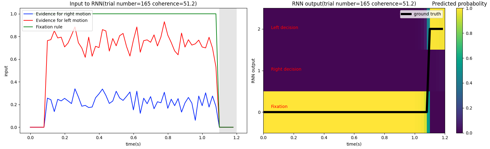
1 2 3 4 5 6 7 8 9 10 11 12 13 14 15 16 17 18 19 20 21 22 23 24 25 26 27 28 29 30 31 32 33 34 i_trial = np.random.choice(200 ) coh = trial_infos[i_trial]['coh' ] print (f'coherence={coh} ' )end = sum ([v for _,v in env.timing.items()])/1000 times = np.arange(end, step=env.dt/1000 ) rules = end - env.timing['decision' ]/1000 , end f, ax = plt.subplots(1 , 2 , figsize=(16 ,5 )) ax[0 ].axvspan(rules[0 ], rules[1 ], facecolor='grey' , alpha=0.2 ) ax[0 ].plot(times, run_inputs[i_trial][:,1 ], 'blue' , label='Evidence for right motion' ) ax[0 ].plot(times, run_inputs[i_trial][:,2 ], 'red' , label='Evidence for left motion' ) ax[0 ].plot(times, run_inputs[i_trial][:,0 ], 'green' , label='Fixation rule' ) ax[0 ].legend(loc='upper left' ) ax[0 ].set_xlabel('time(s)' ) ax[0 ].set_ylabel('input' ) ax[0 ].set_title(f'Input to RNN(trial number={i_trial} coherence={coh} )' ) im = ax[1 ].imshow(softmax(trial_infos[i_trial]['pred' ],axis=-1 ).T, extent=[times[0 ],end,-0.5 ,2.5 ], aspect='auto' , origin='lower' ) ax[1 ].text(0.05 ,0.1 ,'Fixation' , color='r' ) ax[1 ].text(0.05 ,1 ,'Right decision' , color='r' ) ax[1 ].text(0.05 ,2 ,'Left decision' , color='r' ) ax[1 ].plot(times, trial_infos[i_trial]['target' ], 'k' , linewidth=5 , label='ground truth' ) ax[1 ].set_xlabel('time(s)' ) ax[1 ].set_ylabel('RNN output' ) ax[1 ].set_yticks([0 ,1 ,2 ]) ax[1 ].set_title(f'RNN output(trial number={i_trial} coherence={coh} )' ) ax[1 ].legend() cb = plt.colorbar(im, ax=ax[1 ]) cb.ax.set_title('Predicted probabolity' ) plt.tight_layout() plt.show()
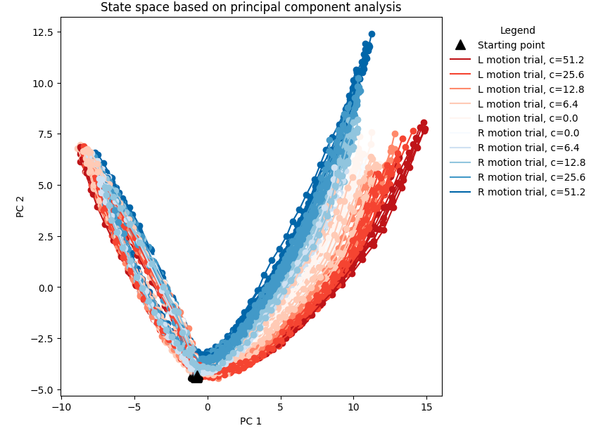
RNN模型测试准确率达到90%以上时,PCA分析不同运动一致比例条件下RNN群体活动轨迹比较容易分开。如果模型的准确率不高,则轨迹比较集中。🦁也就是说,模型是否训练好要设定一个performance threshold~
1 2 3 4 5 6 7 8 9 10 11 12 13 14 15 16 17 18 19 20 21 22 23 24 25 26 27 28 29 30 31 32 33 34 activity = np.concatenate(list (activity_dict[i] for i in range (200 )), axis=0 ) pca = PCA(n_components=3 ) pca.fit(activity) activity_pc = pca.transform(activity) blues = cm.get_cmap('Blues' , len (env.cohs)+1 ) reds = cm.get_cmap('Reds' , len (env.cohs)+1 ) figure = plt.figure(figsize=([7 ,7 ])) for i in range (100 ): activity_pc = pca.transform(activity_dict[i]) trial = trial_infos[i] color_c = blues if trial['ground_truth' ] == 0 else reds color = color_c(np.where(env.cohs == trial['coh' ])[0 ][0 ]) plt.plot(activity_pc[:,0 ], activity_pc[:,1 ], 'o-' , color=color) plt.plot(activity_pc[0 ,0 ], activity_pc[0 ,1 ], '^' , color='black' , markersize=10 ) handles, labels = plt.gca().get_legend_handles_labels() dot = Line2D([], [], marker='^' , label='Starting point' , color='black' , linestyle='None' , markersize=10 ) lines = [] for i_coh, v_coh in reversed (list (enumerate (env.cohs))): line_r = Line2D([], [], label=f'L motion trial, c={v_coh} ' , color=reds(i_coh)) lines.append(line_r) for i_coh, v_coh in enumerate (env.cohs): line_b = Line2D([], [], label=f'R motion trial, c={v_coh} ' , color=blues(i_coh)) lines.append(line_b) handles.extend([dot]+lines) plt.legend(title='Legend' , bbox_to_anchor=(1.4 ,1.0 ), handles=handles, frameon=False ) plt.xlabel('PC 1' ) plt.ylabel('PC 2' ) plt.title('State space based on principal component analysis' ) plt.show()
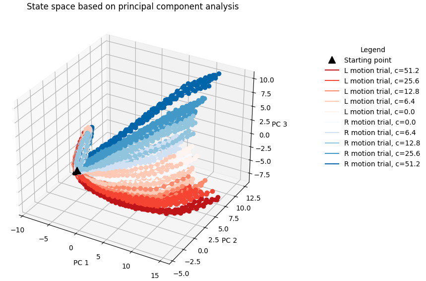
1 2 3 4 5 6 7 8 9 10 11 12 13 14 15 16 17 18 19 20 21 22 23 24 25 26 27 28 29 30 31 32 33 34 35 36 37 from mpl_toolkits.mplot3d import Axes3Dactivity = np.concatenate(list (activity_dict[i] for i in range (200 )), axis=0 ) pca = PCA(n_components=3 ) pca.fit(activity) activity_pc = pca.transform(activity) blues = cm.get_cmap('Blues' , len (env.cohs)+1 ) reds = cm.get_cmap('Reds' , len (env.cohs)+1 ) fig = plt.figure(figsize=([7 ,7 ])) ax = fig.add_subplot(111 , projection='3d' ) for i in range (100 ): activity_pc = pca.transform(activity_dict[i]) trial = trial_infos[i] color_c = blues if trial['ground_truth' ] == 0 else reds color = color_c(np.where(env.cohs == trial['coh' ])[0 ][0 ]) ax.plot(activity_pc[:,0 ], activity_pc[:,1 ], activity_pc[:,2 ], 'o-' , color=color) ax.plot(activity_pc[0 ,0 ], activity_pc[0 ,1 ], activity_pc[0 ,2 ],'^' , color='black' , markersize=10 ) handles, labels = plt.gca().get_legend_handles_labels() dot = Line2D([], [], marker='^' , label='Starting point' , color='black' , linestyle='None' , markersize=10 ) lines = [] for i_coh, v_coh in reversed (list (enumerate (env.cohs))): line_r = Line2D([], [], label=f'L motion trial, c={v_coh} ' , color=reds(i_coh)) lines.append(line_r) for i_coh, v_coh in enumerate (env.cohs): line_b = Line2D([], [], label=f'R motion trial, c={v_coh} ' , color=blues(i_coh)) lines.append(line_b) handles.extend([dot]+lines) ax.set_xlabel('PC 1' ) ax.set_ylabel('PC 2' ) ax.set_zlabel('PC 3' ) ax.set_title('State space based on principal component analysis' ) plt.legend(title='Legend' , bbox_to_anchor=(1.6 ,0.9 ), handles=handles, frameon=False ) plt.show()
补充知识 **kwargs 1 2 3 4 5 6 7 8 9 10 11 kwargs = {'arg1' : 10 , 'arg3' : True , 'arg2' : 'hello' } def example_function (arg1, arg2, arg3 ): print (arg1) print (arg2) print (arg3) example_function(**kwargs)
字典 在Python中,字典是一种可变的数据结构,用于存储键-值对的集合。字典可以使用{}来创建,也可以通过dict()函数创建。update方法可以接受一个字典对象或包含键值对的可迭代对象作为参数,并将其中的键值对添加到调用update方法的字典中。
1 2 3 4 5 6 7 8 9 10 11 12 my_dict = {'key1' : 'value1' , 'key2' : 'value2' } my_dict = dict ( key1 = value1, key2 = value2, ) my_dict = {'key1' : 'value1' , 'key2' : 'value2' } new_dict = {'key3' : 'value3' , 'key4' : 'value4' } my_dict.update(new_dict) print (my_dict)
time.time() 1 2 3 4 5 6 7 import timestart_time = time.time() for i in range (10 ): print (i) end_time = time.time() print (f'程序用时:{end_time-start_time} s' )
参考内容